
광고 한번만 눌러주세요 ㅎㅎ 블로그 운영에 큰 힘이 됩니다.
파이썬에서 한 Figure에서 여러 개로 쪼개서 다양한 그림을 넣고 싶은 경우가 많다.
보통 그래서 필자는 주로 격자 방식으로 한 그림에는 한 주제만 나오게 한다.
그래서 필자가 좋아하는 방법은 평평하게 해 놓고 격자마다 하나씩 나오게 하는 것이다.
import matplotlib.pyplot as plt
from matplotlib.gridspec import GridSpec
import numpy as np
import pickle
with open("./../02/resut.pkl", "rb") as rb :
    result = pickle.load(rb)
하지만 위에 그림에서 왼쪽을 보게 되면, 스케일 자체가 차이가 나서, 실제로 제대로 된 시각화를 할 수가 없게 된다.
그래서 이것을 하는 방법에 대해서 알아보게 되었다.

필자에게는 이러한 그림으로 만들 수 있는 방법이 필요했지만, 지금 기존의 방식으로는 저렇게 만들기 어렵다는 것을 알게 되었다 (> 필자가 조사를 제대로 안 해서 그렇지 될 수도 있다.)
그래서 찾은 방법이 GridSpec이라는 방법을 사용하는 것이다!
fig = plt.figure(figsize=(10, 5))
gs = GridSpec(nrows=2, ncols=2)
## width_ratios=[3, 1], height_ratios=[3, 1]
ax0 = fig.add_subplot(gs[0, 0])
ax1 = fig.add_subplot(gs[1, 0])
ax2 = fig.add_subplot(gs[:, 1])
ax0.plot(result["epoch"],result["aeloss"])
ax1.plot(result["epoch"],result["slloss"])
ax2.plot(result["epoch"],result["auc"])
ax2.plot(result["epoch"],result["teauc"])
plt.show()
이전보다 훨씬 각각에 대해서 잘 보이는 것을 확인하였다.
그리고 각 figure 왼쪽과 오른쪽, 위아래의 스케일을 조정하는 방법은 다음과 같다.
fig = plt.figure(figsize=(10, 5))
##  width_ratios=[3, 1], height_ratios=[3, 1]
gs = GridSpec(nrows=2, ncols=2, width_ratios=[3, 1], height_ratios=[3, 1])
## first
ax0 = fig.add_subplot(gs[0, 0])
## second
ax1 = fig.add_subplot(gs[1, 0])
ax2 = fig.add_subplot(gs[:, 1])
ax0.plot(result["epoch"],result["aeloss"])
ax1.plot(result["epoch"],result["slloss"])
ax2.plot(result["epoch"],result["auc"])
ax2.plot(result["epoch"],result["teauc"])
plt.show()
하지만 필자는 그림을 봐도 각각의 그림에 대해서도 스케일이 크다 보니, 학습이 진행되면서 어떻게 진행되는지가 잘 보이지가 않았다. 머 물론 이런 것 때문에 ylim이나 xlim 같은 방법이 있다는 것은 알고 있다.
하지만 먼가 좀 더 멋지게 그려보고 싶은 마음이 있어서 찾아보니 이런 게 있었다.
바로 add_axes를 사용하는 것이었다.
fig.add_axes([0.43, 0.6, 0.15, 0.15])
#[lowerCorner_x, lowerCorner_y, width, height]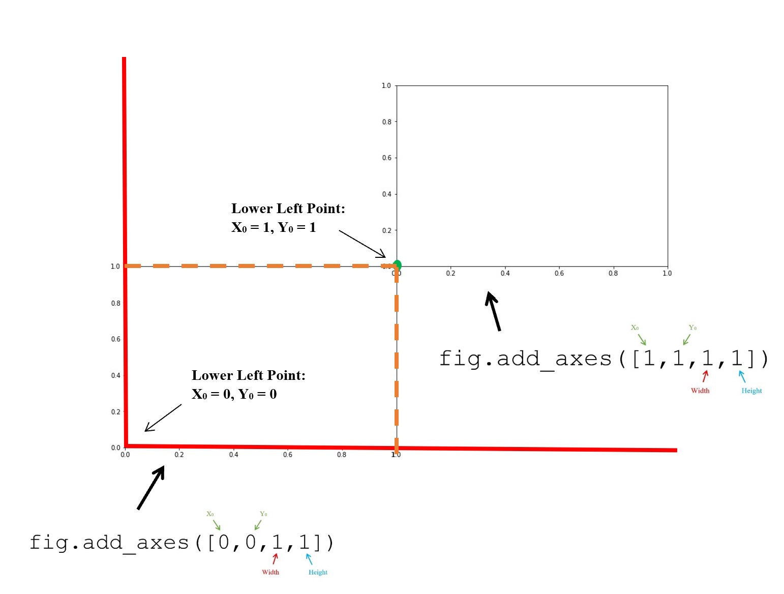
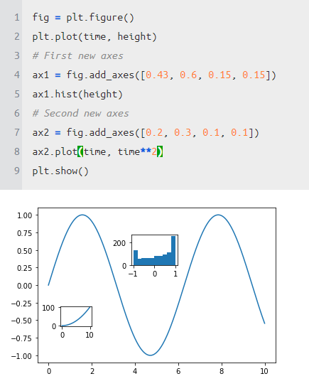
fig = plt.figure(figsize=(10, 5))
gs = GridSpec(nrows=2, ncols=2)
## first
ax0 = fig.add_subplot(gs[0, 0])
## second
ax1 = fig.add_subplot(gs[1, 0])
ax2 = fig.add_subplot(gs[:, 1])
ax0.plot(result["epoch"],result["aeloss"])
ax1.plot(result["epoch"],result["slloss"])
ax2.plot(result["epoch"],result["auc"])
ax2.plot(result["epoch"],result["teauc"])
ax3 = fig.add_axes([0.2, 0.6, 0.2, 0.2])
ax3.plot(result["epoch"],result["aeloss"])
ck = result["aeloss"][-3:] + result["aeloss"][-3:]
ax3.set_xlim(result["epoch"][-3],result["epoch"][-1])
ax3.set_ylim(np.min(ck), np.max(ck))
ax4 = fig.add_axes([0.65, 0.4, 0.25, 0.25])
ax4.plot(result["epoch"],result["auc"])
ax4.plot(result["epoch"],result["teauc"])
ck = result["teauc"][-3:] + result["auc"][-3:]
ax4.set_xlim(result["epoch"][-3],result["epoch"][-1])
ax4.set_ylim(np.min(ck), np.max(ck))
plt.show()
마지막 부분을 잘 보니, 역시 평평해 보이지만, 위로 갔다 아래로 갔다 하는 것을 확인할 수 있습니다.
하지만 먼가 저 빨간 화살표처럼 실제로 어떤 부분을 나타내는지가 있다면 더욱 좋을 것 같습니다.
최근에 사실 필자도 이러한 그림을 보고 따라 하고 싶었는데, 딱 맞는 것을 찾게 되었습니다.

from mpl_toolkits.axes_grid1.inset_locator import inset_axes, mark_inset바로 inset_axes와 mark_inset을 사용하는 것이다.
fig = plt.figure(figsize=(10, 5))
gs = GridSpec(nrows=2, ncols=2)
ax0 = fig.add_subplot(gs[0, 0])
ax1 = fig.add_subplot(gs[1, 0])
ax2 = fig.add_subplot(gs[:, 1])
ax0.plot(result["epoch"],result["aeloss"])
ax1.plot(result["epoch"],result["slloss"])
ax2.plot(result["epoch"],result["auc"])
ax2.plot(result["epoch"],result["teauc"])
#############
axins = inset_axes(ax0, "100%", "100%", bbox_to_anchor=[0.2, 0.2, 0.4, 0.4],
                   bbox_transform=ax0.transAxes, borderpad=0)
axins.plot(result["epoch"],result["aeloss"])
ck = result["aeloss"][-3:]
xlims = (result["epoch"][-3],result["epoch"][-1])
ylims = (np.min(ck), np.max(ck))
axins.set(xlim=xlims, ylim=ylims)
mark_inset(ax0, axins, loc1=1, loc2=3, fc="none", ec="0.5")
##########3
axins = inset_axes(ax2, "100%", "100%", bbox_to_anchor=[0.2, 0.3, 0.4, 0.4],
                   bbox_transform=ax2.transAxes, borderpad=0)
axins.plot(result["epoch"],result["auc"])
axins.plot(result["epoch"],result["teauc"])
ck = result["teauc"][-3:] + result["auc"][-3:]
xlims = (result["epoch"][-3],result["epoch"][-1])
ylims = (np.min(ck), np.max(ck))
axins.set(xlim=xlims, ylim=ylims)
ck = result["aeloss"][-3:] + result["aeloss"][-3:]
mark_inset(ax2, axins, loc1=1, loc2=4, fc="none", ec="0.5")

plt.show()
해당 그림에서는 잘 나오는 것 같지만, 조금 문제가 있었다.
예제 그림을 보면 다음과 같다.
from mpl_toolkits.axes_grid1.inset_locator import inset_axes, mark_inset
fig = plt.figure(figsize=(10, 5))
gs = GridSpec(nrows=2, ncols=2)
ax = fig.add_subplot(gs[:,0])
ax.plot(time, score)
ax1 = fig.add_subplot(gs[0,1])
ax1.plot(time , height)
ax2 = fig.add_subplot(gs[1,1])
ax2.plot(time , height)
axins = inset_axes(ax2, "100%", "100%", bbox_to_anchor=[0.36, .5, .2, .2],
                   bbox_transform=ax2.transAxes, borderpad=0)
axins.plot(time, height)
axins.set(xlim=(6,8)) # , ylim=(-1,1)
mark_inset(ax2, axins, loc1=2, loc2=3, fc="none", ec="0.5")
plt.show()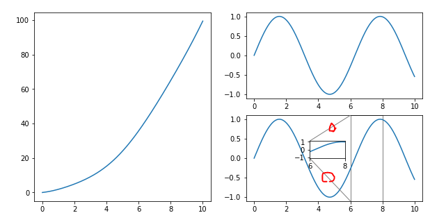
안에 있는 선이 먼가 반대쪽으로 되어야 하는데, 이러쿵저러쿵해도 잘 안된다.
그래서 다른 글을 참고하여서 하니 잘 작동하였다.
def my_mark_inset(parent_axes, inset_axes, loc1a=1, loc1b=1, loc2a=2, loc2b=2, **kwargs):
    rect = TransformedBbox(inset_axes.viewLim, parent_axes.transData)
    pp = BboxPatch(rect, fill=False, **kwargs)
    parent_axes.add_patch(pp)
    p1 = BboxConnector(inset_axes.bbox, rect, loc1=loc1a, loc2=loc1b, **kwargs)
    inset_axes.add_patch(p1)
    p1.set_clip_on(False)
    p2 = BboxConnector(inset_axes.bbox, rect, loc1=loc2a, loc2=loc2b, **kwargs)
    inset_axes.add_patch(p2)
    p2.set_clip_on(False)
    return pp, p1, p2
from mpl_toolkits.axes_grid1.inset_locator import inset_axes, mark_inset
import matplotlib.patches as mpatches
from mpl_toolkits.axes_grid1.inset_locator import (inset_axes, TransformedBbox,
BboxPatch, BboxConnector)
fig = plt.figure(figsize=(10, 5))
gs = GridSpec(nrows=2, ncols=2)
ax = fig.add_subplot(gs[:,0])
ax.plot(time, score)
ax1 = fig.add_subplot(gs[0,1])
ax1.plot(time , height)
ax2 = fig.add_subplot(gs[1,1])
ax2.plot(time , height)
axins = inset_axes(ax2, "100%", "100%", bbox_to_anchor=[0.36, .5, .2, .2],
bbox_transform=ax2.transAxes, borderpad=0)
axins.plot(time, height)
xlims = (7,9)
ylims = (-1,1)
axins.set(xlim=xlims, ylim=ylims)
my_mark_inset(ax2, axins, loc1a=1, loc1b=2, loc2a=4, loc2b=3, fc="none", ec="0.5") #
plt.show()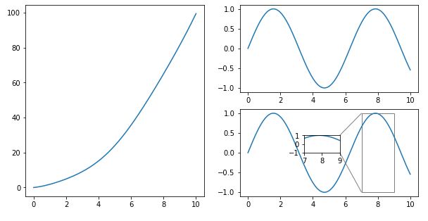
여기서는 subplots를 나눌 때 합치는 방법과 중요 부분을 확인하는 방법에 대해서 알아봤다.
추가로 각 subplot마다 그리는 것이 귀찮으니 함수로 만들려고 하는데, 고려할 사항이 너무 많아 포기했다.
일단 공유
def subplotting(ax , store , x , y ,cond={}, **kwargs) :
    ax.plot(store[x],store[y],**kwargs)
    if "ylabel" in cond :
        ax.set_ylabel(cond["ylabel"], fontsize= 10)
    if "xlabel" in cond :
        ax.set_xlabel(cond["xlabel"], fontsize= 10)
    if "xlim" in cond :
        ax.set_xlim(cond["xlim"])
    if "ylim" in cond :
        ax.set_ylim(cond["ylim"])
    if "title" in cond :
        ax.set_title(cond["title"], fontsize= 15)
    ax.legend()
    return ax
위의 코드는 제 github에 있습니다.
sungreong/Blog
Blong Code. Contribute to sungreong/Blog development by creating an account on GitHub.
github.com
# Plot Organization in matplotlib — Your One-stop Guide If you are reading this, it is probably…
A brief tutorial on how to organize multiple subplots with different positions and sizes on matplotlib to save editing time.
towardsdatascience.com
https://github.com/matplotlib/matplotlib/issues/12323/
indicate_inset_zoom sometimes draws incorrect connector lines · Issue #12323 · matplotlib/matplotlib
Bug report Bug summary Depending on location of inset, the connector lines are not drawn to the nearest two corners. Code for reproduction import matplotlib.pyplot as plt import numpy as np line=np...
github.com
'분석 Python > Visualization' 카테고리의 다른 글
| Matplotlib 한글폰트 사용하는 전체 또는 개별 적용하는 방법 (0) | 2020.04.03 |
|---|---|
| subplotting을 위한 plot 함수 만들어서 코드 간단하게 하기 (0) | 2020.03.29 |
| [ Python ] (범례 순서 변경) change legend order (0) | 2020.02.06 |
| [ Python ] density plot과 count ratio plot 그리기 (0) | 2020.02.01 |
| [ Python ] 유용한 시각화 함수들 모음 (boxplot, scatter plot, plotly.express, etc) (0) | 2020.01.14 |