https://towardsdatascience.com/how-dis-similar-are-my-train-and-test-data-56af3923de9b
How (dis)similar are my train and test data?
Understanding a scenario where your machine learning model can fail
towardsdatascience.com
해당 내용이 굉장히 흥미로워서 공유를 하면서 나도 연습을 해보려고 작성했다.
흥미로운 이유는 만약 train으로 함수를 추정하고 test로 평가했을 때 성능이 안좋은 이유는 우리는 보통 overfitting이 발생했다고 한다.
하지만 이 글에서는 그 문제일수도 있지만, 새로운 문제를 제기한다.
실제 train 분포와 test분포가 다르다면 안되지 않을까?
이 글에서 예를 든 것은 train으로 학습을 했을 때 나이가 중요하다고 하자.
그런데 train에서는 젊은 사람만 있고, test에는 노인만 있는 데이터가 모였을 때? 과연 우리가 학습한 모형이
전혀 새로운 패턴이 나오는 것이므로 예측이 잘 안되는게 당연하지않을까? 에대해서 말한다.
나도 보다보니 공감을 하게 되었다. 실제로 시기가 다른 데이터를 사용했을 때 어떤 시기에서는 잘 예측이 되지만 다음 시기에서는 그 예측이 잘 안맞는 경우가 있다. 이럴 때 overfitting 보다는 분포 자체가 달라서 안되는지도 의심해 볼수도 있을 것 같다.
그래서 저자는 이러한 부분을 Covariate Shift 이 발생했다고 한다.
내가 알고 있던 covariate shift 같은 경우 NN에서 Weight에서 몇몇 가중치가 평균보다 커서 weight 의 분포자체가 달리지는 문제라고 하고 그럴 때 보통 Batch Normalization을 쓴다고 한다.
그래서 여기서는 다음과 같은 방법으로 진행을 한다.
처음에는 target(isFraud)를 빼고 기존에는 합쳐져 있으니 일단 분리하는 것을 진행하자.
test_size = 0.3
shuffle = True
random_state = None
from sklearn.model_selection import train_test_split

df_y = df["isFraud"]
df_x = df.drop("isFraud", axis =1)
X_train, X_test , y_train, y_test =\
train_test_split(df_x , df_y , test_size=test_size, random_state=random_state, shuffle=shuffle)
그렇다면 우리가 여기서 드는 생각이 다음과 같다.
> 여기서 나눈 train 과 test가 같은 분포를 따를까?
나도 이글을 보고 실제로 그러한 부분에 대해서는 체크를 한번도 안해본 내 자신이 생각났다.
그래서 여기서는 다음과 같이 train에는 1을 주고 test에는 0을 주는 다른 target변수를 부여한다.
그다음에 이 둘을 다시 합친다. 그리고 새로만든 target과 input을 분리한다.
X_test["is_train"] = 0
X_train["is_train"] = 1
df_combine = pd.concat([X_train, X_test], axis=0, ignore_index=True)
y = df_combine['is_train'].values
x = df_combine.drop('is_train', axis=1).values
그런 다음 그것을 Classifier하는 모델링을 한다.
여기서는 좀 더 코드를 빨리 돌리기 위해서 multiprocessing으로 해봤다( 실제로 해보니 조금 빠른 듯하다)
tst, trn = X_test.values, X_train.values
m = RandomForestClassifier(n_jobs= -1 , max_depth=5, min_samples_leaf = 5)
predictions = np.zeros(y.shape)
skf = SKF(n_splits=20, shuffle=True, random_state=100)

## https://nzw0301.github.io/2016/02/multiprocessing-paralell
## multiprocessing sklearn
def prob_one_fold(train_idx , test_idx) :
    X_train_fold , X_test_fold = x[train_idx], x[test_idx]
    y_train_fold , y_test_fold = y[train_idx], y[test_idx]
    m.fit(X_train_fold , y_train_fold )
    probs = m.predict_proba(X_test_fold)[:, 1] #calculating the probability
    #predictions[test_idx] = probs
    Output = pd.DataFrame([test_idx , probs]).T
    return Output

Pred = Parallel(n_jobs=3)\
(delayed(prob_one_fold)(train_idxs, test_idxs)\
 for train_idxs, test_idxs in skf.split(x, y))

 OUT = pd.concat(Pred,axis = 0)
 OUT.columns = ["idx", "p"]
 OUT.sort_values(by = ["idx"] , inplace = True)
OUT.reset_index(drop= True , inplace = True)
predictions = OUT["p"].values
from sklearn.metrics import roc_auc_score as AUC
print("ROC-AUC for train and test distributions:", AUC(y, predictions))
여기서 그러면 AUC 0.5가 나왔다
그렇다면 여기서의 AUC의 의미는 뭐냐? 바로 Train인지 test인지 분류하는 AUC이다.
여기서는 그 값을 0.5로 줬다는 것은 구분할 수 없다는 것과 같다.
결국 그래서 여기서는 강한 Covariate shift가 있다라고 말한 근거가 없는 것이다!
그다음에는 내가 하진 않았지만 medium에서는 다음과 같은 이야기를 또 진행한다.
여기서 test data에 대해서 향상시킬려면 어떻게 해야할지?
- Dropping of drifting features
- Importance weight using Density Ratio Estimation
1번 Dropping of drifting features
1.1 이전에 모델링 한 것에서 feature importance plotting을 해보라
features    = X_train.columns.tolist()
importances = m.feature_importances_
indices     = np.argsort(importances)
plt.title('Feature Importances')
color = np.random.choice(sorted_names, len(features) , replace = False)
plt.barh(range(len(indices)), importances[indices], color=color, align='center')
plt.yticks(range(len(indices)), [features[i] for i in indices])
plt.xlabel('Relative Importance')s
plt.show()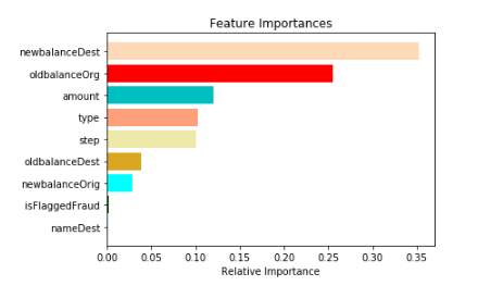
1.2 만약 AUC가 높게 나온다면 위에 상위에 있는 Feature가 분명 문제를 발생시키고 있는 것이다.
1.3 그것들을 하나씩 빼서 다시 모델링을 해봐라 그렇게 해서 성능이 떨어지지 않을 때 까지의 feature를 모아라
여기서 성능이 떨어지지 않는 다는 의미는 AUC가 안내려갈정도로 까지 해보라는 의미일 것이다.(왜냐면 그런 놈들은 driftting이나 covariate shift를 발생시키는 변수니까 말이다)
이런 식으로 하면 train과 test를 혼란스럽게 한 변수를 제거하므로 더 나은 성능을 만들 수 있을 것이다!

2. Importance weight using Density Ratio Estimation
- 이 방법은 covariate shift가 존재하든 존재하지 않든 상관없이 적용 할 수 있는 방법이다!
- 한 값의 예측값을 한번 보자. 이 확률은 우리에게 말해주는 것이다 있다.
- 이 확률은 우리의 모델에 따라서 이 데이터가 train data에 속 할 확률 인 것이다.
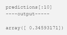
- 여기서는 0.34라고 나온다 이것을 P(train)라고 하자. 그렇다면 반대는 test에 속할 확률이나 P(test)라고 하자.
- 여기서 magick trick 방법이라고 하는 방법을 쓴다!
- w = P(test) / P(train) 으로 정의!!!!
- 이 w는 train data로부터 test데이터가 얼마나 가까운지를 나타낸다!!!
- 만약 이 관측치에서 w가 커지면 test data 가깝다는 의미다.
- 이것은 직관적으로 우리의 모델이 패턴을 test data 에서 잘 맞추려고 한다는 것임을 알 수 있다고 한다!
- We can use this w as sample weights in any of our classifier to increase the weight of these observation which seems similar to our test data.
- Intuitively this makes sense as our model will focus more on capturing patterns from the observations which seems similar to our test.
import matplotlib.pyplot as plt
import seaborn as sns
plt.figure(figsize=(20,5))
predictions_train = predictions[len(tst):] #filtering the actual training rows
weights = (1/predictions_train) -1
weights /= np.mean(weights) # Normalizing the weights
plt.xlabel("Computed sample weight")
plt.ylabel("# Samples")
sns.distplot(weights, kde=False)
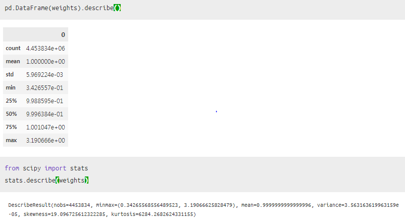
- 만약 이 Plot이 높은 값에 나왔다면 패턴을 test data에 더 유사하다는 것을 알 수 있다!
- 그래서 현재 데이터에서는 train data기준으로 봤을 때, 거의 1에 가깝다는 것을 알 수 있고,
- 따라서 이 데이터는 train또는 test 지역에 상관없이 feature가 나온다는 것을 의미한다!
나의 결론!
- 이런식으로 overfit이 났을 때 이러한 고민을 해보지 않았는데, 적용할 가치가 충분히 있다고 생각한다!
- 우리가 일반적으로 샘플링을 임의로 나누는데, 이럴 때 잘 나눠질 떄의 기준점을 만들 수 있다!
- 아무리해도 잘 나눠지지 않았을 때, 그렇다면 covariate shift 변수를 제거함으로써 모델 성능을 향상 시킬 수 있는 방향으로 할 수 있을 것 같다.
- 그리고 마지막에 이런 train , test 자체의 패턴을 통해서 train data 기준에서 이 놈의 magick trick (w)가 1보다 높게 나와서 test data를 나오는지를 확인해서 어디 feature에서 나오는지 알 수 있다!
'관심있는 주제 > 분석 고려 사항' 카테고리의 다른 글
| PySyft and the Emergence of Private Deep Learning -?? (0) | 2019.06.08 |
|---|---|
| 어떻게 언제 왜 Normalize Standardize Rescale 해주는지??! (3) | 2019.05.18 |
| Feature engineering ( 글 리뷰 및 내 생각 ) (0) | 2019.05.06 |
| Design Thinking에 대하여 (0) | 2019.05.06 |
| threshold는 어떻게 정해야 할까? 개인적인 간단한 생각 (0) | 2019.05.04 |