728x90
이번에는 histplot에 대해서 정리해보려고 한다.
확률 값을 density plot으로 표현하는 것보다 오히려 histogram으로 bins를 여러 개 쪼개는 것도 효과적이라는 생각을 가지게 되었기 때문이고 이것에 대해서 정리해보고자 한다.
import seaborn as sns
import matplotlib.pyplot as plt
penguins = sns.load_dataset("penguins")
sns.histplot(data=penguins, x="flipper_length_mm")
bins 추가
fig, axes = plt.subplots(nrows=2, ncols=1)
axes = axes.flatten()
sns.histplot(data=penguins, x="flipper_length_mm",ax=axes[0])
sns.histplot(data=penguins, x="flipper_length_mm",ax=axes[1],bins=100)
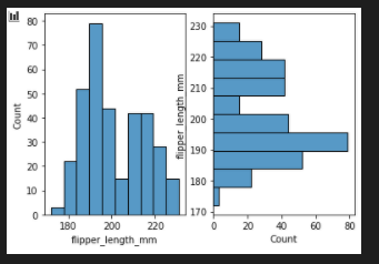
flip the plot
fig, axes = plt.subplots(nrows=1, ncols=2)
axes = axes.flatten()
sns.histplot(data=penguins, x="flipper_length_mm",ax=axes[0])
sns.histplot(data=penguins, y="flipper_length_mm",ax=axes[1])
add bin width
fig, axes = plt.subplots(nrows=1, ncols=2)
axes = axes.flatten()
sns.histplot(data=penguins, x="flipper_length_mm",ax=axes[0],binwidth=3)
sns.histplot(data=penguins, x="flipper_length_mm",ax=axes[1],binwidth=10)
add kde
fig, axes = plt.subplots(nrows=1, ncols=2)
axes = axes.flatten()
sns.histplot(data=penguins, x="flipper_length_mm",ax=axes[0])
sns.histplot(data=penguins, x="flipper_length_mm",ax=axes[1],kde=True)
multiple histogram
sns.histplot(data=penguins)add hue & multiple
multiple
- stack
- layer
- dodge
- fill
fig, axes = plt.subplots(nrows=2, ncols=2)
axes = axes.flatten()
sns.histplot(data=penguins, x="flipper_length_mm", hue="species", multiple="stack",ax=axes[0])
sns.histplot(data=penguins, x="flipper_length_mm", hue="species", multiple="layer",ax=axes[1])
sns.histplot(data=penguins, x="flipper_length_mm", hue="species", multiple="dodge",ax=axes[2])
sns.histplot(data=penguins, x="flipper_length_mm", hue="species", multiple="fill",ax=axes[3])
add step
- bar
- step
- ploy
fig, axes = plt.subplots(nrows=1, ncols=2)
axes = axes.flatten()
sns.histplot(data=penguins, x="flipper_length_mm", hue="species", multiple="stack",ax=axes[0], element="step")
sns.histplot(data=penguins, x="flipper_length_mm", hue="species", multiple="layer",ax=axes[1], element="step")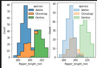
add element
- poly
- bars
- step
fig, axes = plt.subplots(nrows=3, ncols=1)
axes = axes.flatten()
sns.histplot(penguins, x="flipper_length_mm", hue="species", element="bars",ax=axes[0])
sns.histplot(penguins, x="flipper_length_mm", hue="species", element="poly",ax=axes[1])
sns.histplot(penguins, x="flipper_length_mm", hue="species", element="step",ax=axes[2])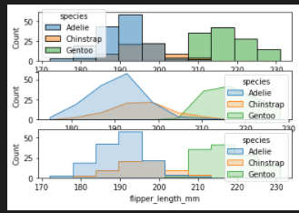
add stat
- probability
- density
- frequency
- count
fig, axes = plt.subplots(nrows=4, ncols=1,figsize=(12,6))
axes = axes.flatten()
sns.histplot(penguins, x="flipper_length_mm", hue="species",ax=axes[0],stat="probability")
sns.histplot(penguins, x="flipper_length_mm", hue="species", ax=axes[1],stat="density")
sns.histplot(penguins, x="flipper_length_mm", hue="species", ax=axes[2],stat="frequency")
sns.histplot(penguins, x="flipper_length_mm", hue="species", ax=axes[3],stat="count")

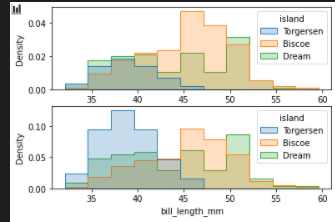
stat=density / common_norm
fig, axes = plt.subplots(nrows=2, ncols=1)
axes = axes.flatten()
sns.histplot(
    penguins, x="bill_length_mm", hue="island", element="step",
    stat="density", common_norm=True,ax=axes[0]
)
sns.histplot(
    penguins, x="bill_length_mm", hue="island", element="step",
    stat="density", common_norm=False,ax=axes[1]
)
stat=probability/ discrete
tips = sns.load_dataset("tips")
fig, axes = plt.subplots(nrows=2, ncols=1,figsize=(12,6))
axes = axes.flatten()
sns.histplot(data=tips, x="size", stat="probability", discrete=False,ax=axes[0])
sns.histplot(data=tips, x="size", stat="probability", discrete=True,ax=axes[1])
add shrink
tips = sns.load_dataset("tips")
fig, axes = plt.subplots(nrows=2, ncols=1,figsize=(12,6))
axes = axes.flatten()
sns.histplot(data=tips, x="day", shrink=.8,ax=axes[0])
sns.histplot(data=tips, x="day", shrink=1.0,ax=axes[1])
add hue / multiple = "dodge"
tips = sns.load_dataset("tips")
fig, axes = plt.subplots(nrows=2, ncols=1,figsize=(12,6))
axes = axes.flatten()
sns.histplot(data=tips, x="day", hue="sex", multiple="dodge", shrink=.8,stat="probability",ax=axes[0])
sns.histplot(data=tips, x="day", hue="sex", multiple="dodge", shrink=.8,stat="count",ax=axes[1])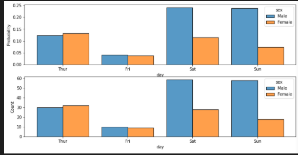
pred_np = np.array([0,1,1,1,0])
label_np = np.array([1,0,1,0,0])
prop_table = pd.DataFrame(np.hstack([pred_np,label_np]),
columns=["pred","true"])
prop_table["true"] = prop_table["true"].astype("str")
sns.histplot(data=prop_table,x="true", hue="pred", multiple="fill",
shrink=0.8,stat="count",common_norm=False)
plt.show()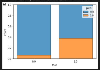
add log_scale
planets = sns.load_dataset("planets")
fig, axes = plt.subplots(nrows=2, ncols=1,figsize=(12,6))
axes = axes.flatten()
sns.histplot(data=planets, x="distance", log_scale=False ,ax=axes[0])
sns.histplot(data=planets, x="distance", log_scale=True ,ax=axes[1])
add fill
planets = sns.load_dataset("planets")
fig, axes = plt.subplots(nrows=2, ncols=1,figsize=(12,6))
axes = axes.flatten()
sns.histplot(data=planets, x="distance", log_scale=True ,ax=axes[0],fill=False)
sns.histplot(data=planets, x="distance", log_scale=True ,ax=axes[1],fill=True)
add cumulative
fig, axes = plt.subplots(nrows=2, ncols=1,figsize=(12,6))
axes = axes.flatten()
sns.histplot(
    data=planets, x="distance", hue="method",
    hue_order=["Radial Velocity", "Transit"],
    log_scale=True, element="step", fill=True,
    cumulative=True, stat="density", common_norm=False,
    ax =axes[0]
)
sns.histplot(
    data=planets, x="distance", hue="method",
    hue_order=["Radial Velocity", "Transit"],
    log_scale=True, element="step", fill=True,
    cumulative=False, stat="density", common_norm=False,
    ax =axes[1]
)
2d histogram
sns.histplot(penguins, x="bill_depth_mm", y="body_mass_g")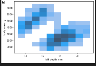
The bivariate histogram / add hue
fig, axes = plt.subplots(nrows=1, ncols=2,figsize=(12,6))
axes = axes.flatten()
sns.histplot(penguins, x="bill_depth_mm", y="body_mass_g", ax=axes[0])
sns.histplot(penguins, x="bill_depth_mm", y="body_mass_g", hue="species",ax=axes[1])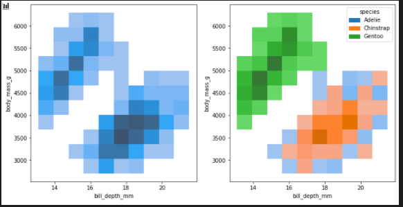
Multiple color maps / add bins
fig, axes = plt.subplots(nrows=1, ncols=3,figsize=(12,6))
axes = axes.flatten()
sns.histplot(
    penguins, x="bill_depth_mm", hue="species", legend=False,
    ax =axes[0]
)
sns.histplot(
    penguins, x="bill_depth_mm", y="species", hue="species", legend=False,
    ax=axes[1], bins=100
)
sns.histplot(
    penguins, x="bill_depth_mm", y="species", hue="species", legend=False,
    ax=axes[2], bins=10
)
The bivariate histogram
fig, axes = plt.subplots(nrows=1, ncols=4,figsize=(18,6))
axes = axes.flatten()
sns.histplot(
    planets, x="year", y="distance",
    bins=30, discrete=(True, False), log_scale=(False, True),
    ax =axes[0]
)
sns.histplot(
    planets, x="year", y="distance",
    bins=30, discrete=(True, False), log_scale=(False, True),
    thresh=None,
    ax =axes[1]
)
sns.histplot(
    planets, x="year", y="distance",
    bins=30, discrete=(True, False), log_scale=(False, True),
    pthresh=.05, pmax=.9,
    ax = axes[2]
)
sns.histplot(
    planets, x="year", y="distance",
    bins=30, discrete=(True, False), log_scale=(False, True),
    cbar=True, cbar_kws=dict(shrink=.75),
    ax=axes[3]
)
code
import plotly.express as px
df = px.data.tips()
fig = px.histogram(df, x="total_bill")
fig.show()

import plotly.express as px
df = px.data.tips()
# Here we use a column with categorical data
fig = px.histogram(df, x="day")
fig.show()
import plotly.express as px
import numpy as np

df = px.data.tips()
# create the bins
counts, bins = np.histogram(df.total_bill, bins=range(0, 60, 5))
bins = 0.5 * (bins[:-1] + bins[1:])

fig = px.bar(x=bins, y=counts, labels={'x':'total_bill', 'y':'count'})
fig.show()
import plotly.express as px
df = px.data.tips()
fig = px.histogram(df, x="total_bill", histnorm='probability density')
fig.show()
import plotly.express as px
df = px.data.tips()
fig = px.histogram(df, x="total_bill",
                   title='Histogram of bills',
                   labels={'total_bill':'total bill'}, # can specify one label per df column
                   opacity=0.8,
                   log_y=True, # represent bars with log scale
                   color_discrete_sequence=['indianred'] # color of histogram bars
                   )
fig.show()
import plotly.express as px
df = px.data.tips()
fig = px.histogram(df, x="total_bill", color="sex")
fig.show()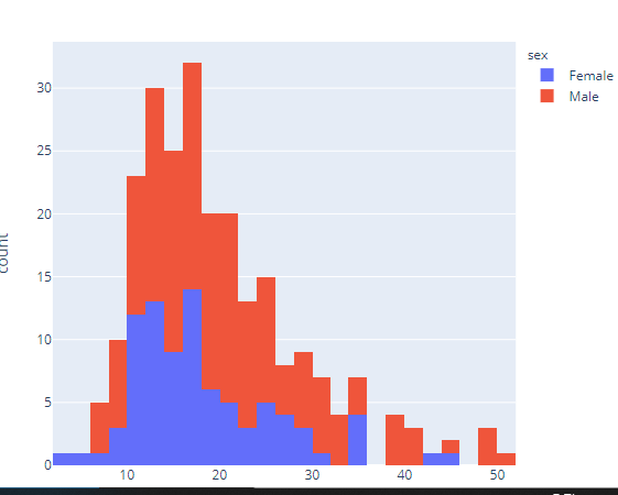
import plotly.express as px
df = px.data.tips()
fig = px.histogram(df, x="total_bill", y="tip", histfunc='avg')
fig.show()
import plotly.express as px
df = px.data.tips()
fig = px.histogram(df, x="total_bill", color="sex", marginal="rug", # can be `box`, `violin`
                         hover_data=df.columns)
fig.show()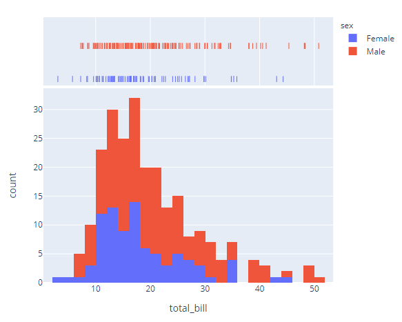
Histograms
How to make Histograms in Python with Plotly.
plotly.com
seaborn.pydata.org/generated/seaborn.histplot.html
seaborn.histplot — seaborn 0.11.1 documentation
Like thresh, but a value in [0, 1] such that cells with aggregate counts (or other statistics, when used) up to this proportion of the total will be transparent.
seaborn.pydata.org
'분석 Python > Visualization' 카테고리의 다른 글
| [ Python ] jpg, png 를 gif 또는 mp4로 만들기 (0) | 2022.05.22 |
|---|---|
| pybaobabdt) DT Tree Visualization 해보기 (0) | 2021.12.18 |
| python) treemap 알아보기 (0) | 2021.04.29 |
| [Visualization] Learning Curve를 이용하여 시각화하기(Train/Valid) (0) | 2020.12.18 |
| [Visualization] keras 결과물(history) 시각화하는 함수 (0) | 2020.11.21 |