
광고 한번만 눌러주세요 ㅎㅎ 블로그 운영에 큰 힘이 됩니다.
실제 분석 시에 정형 데이터의 범주형 데이터 처리가 골치가 아픕니다.
범주형 데이터는 보통 one-hot을 통해, 데이터를 굉장히 희소하게(sparse)하게 만들기 때문입니다.
보통 이렇게 차원이 커지게 되면, 차원의 저주에 빠질 수 있으면서, 학습도 굉장히 잘 안됩니다.
그래서 저는 보통 차원이 커질 경우 보통 embedding을 시키거나, 아니면 요즘은 catboost encoder나, target encoder 같은 방법을 써보려고 합니다.

이번에는 좀 더 변수 선택 차원으로 이야기해보고자
Chi-square 독립 검정을 통해 변수 선택을 하는 것을 보게 되어, 해보면서 공유합니다.
Chi-Square Test of Independence
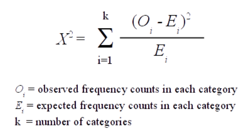
카이 제곱 독립 검정은 보통 두 범주형(명목형) 변수 사이에 유의미한 관계가 있는지 아닌지를 검정합니다.
보통 카이 제곱 독립 검정은 가설 검정을 통해서 하게 됩니다.
귀무 가설$H_0$ : 두 변수들 간에는 관계가 없다
대립 가설$H_1$ : 두 변수들 간에는 관계가 있다.
다른 통계적 검정처럼 P-value를 이용해서 할 수 있습니다.
만약 p-value가 유의미하다면, 귀무가설을 기각할 수 있습니다.
해석은 두 변수들 간에 관계가 없다고 할 수 없다? 정도로 합니다.
만약 p-value가 유의미하지 않다면, 귀무가설을 기각할 수 없다고 합니다.
해석은 두 변수들 간에 관계가 없다고 할만한 근거가 없다.
이번에 실험한 것은 전에 소개했던 xverse 패키지(url)에 있는 MonotonicBinning을 사용해서 연속형은 모두 binning을 하고 변수 선택을 통해 성능 차이가 있는지 보겠습니다.
일단 성능 차이를 보기 전에 카이 제곱 검정을 하기 위해서는 crosstab모양으로 만들어야 합니다. 그래서 다음과 같은 pandas 함수를 쓰면 됩니다.

from scipy.stats import chi2_contingency
chi_res  = chi2_contingency(pd.crosstab(out_X['EDUCATION'], y))
print('Chi2 Statistic: {}, p-value: {}'.format(chi_res[0], chi_res[1]))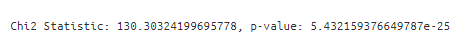
이런 식으로 아주 편리하게 도출해줍니다. 그러면 여기서 나온 p-value를 바탕으로 귀무 가설 기각 여부를 결정합니다.
import numpy as np
import pandas as pd
from xverse.feature_subset import FeatureSubset
from xverse.transformer import MonotonicBinning
from xverse.feature_subset import SplitXY

fac_var = [ 'SEX','EDUCATION','MARRIAGE']
target_var = ['default payment next month']

df[fac_var] = df[fac_var].astype("category")
test[fac_var] = test[fac_var].astype("category")

clf = SplitXY(target_var) #Split the dataset into X and y
X, y = clf.fit_transform(df) #returns features (X) dataset and target(Y) as a numpy array
testX, testy = clf.transform(test)

clf = MonotonicBinning()
clf.fit(X, y)

out_X = clf.transform(X)
test_X = clf.transform(testX)

for col in out_X.columns.tolist() :
    out_X[col] = out_X[col].cat.add_categories("missing").fillna("missing")
    test_X[col] = test_X[col].cat.add_categories("missing").fillna("missing")
이제 재료는 준비를 했으니, 한번 가설 검정을 해보겠습니다.
chi2_check = []
for i in out_X.columns.tolist():
    if chi2_contingency(pd.crosstab(y, out_X[i]))[1] < 0.05:
        chi2_check.append('Reject Null Hypothesis')
    else:
        chi2_check.append('Fail to Reject Null Hypothesis')
res = pd.DataFrame(data = [out_X.columns.tolist(), chi2_check]
             ).T
res.columns = ['Column', 'Hypothesis']
print(res)
지금 보면 모두 귀무가설을 기각할 수 있다고 나옵니다, 모두 변수 y랑 관계가 있다고 나옵니다
Post Hoc Testing
카이-제곱 독립성 검정은 데이터를 전체적으로 테스트한다는 것을 의미하는 옴니버스 검정입니다.
만약 한 범주 안에 여러 개의 클래스를 가지고 있다면, 즉 카이-제곱 테이블이 2 × 2보다 클 경우, 우리는 어떤 형상의 답과의 관계를 잘 알 수 없을 것입니다.
그러므로 어떤 계급이 정확히 영향이 있는지 알려면 우리는 Post Hoc Testing이 필요합니다.
다중 2x2 카이제곱 독립성 검정을 하기 위해서는 한 범주에서 여러 개의 클래스를 다 나눠줘야 합니다.
즉 이것은 아시다시피 OneHotEncoding입니다!


그러나 기억해야 할 것이 있습니다. 다중 클래스를 서로에 대해서 비교할 때는 각 테스트의 false positive의 혼합된 오류율을 의미합니다.
예를 들어, 처음 검정 시 0.05의 p-value를 가진다면, false positive 가 5% 가능성이 있다는 것이고, 만약 3개의 페어가 있다고 했을 때 계속 검정 시 총 15%까지 될 수 있습니다. 이것은 굉장히 p-value에서는 높은 수치입니다.
이러한 경우에, Bonferroni-adjusted method를 사용한다고 합니다.
adjust $p-value = \frac{p}{N}$
$N$ 한 범주의 고유의 수 (유니크한 수) 예) 성별-> N:2(최소)
bon_p_value = 0.05/out_X[i].nunique()이제 그러면 각 범주마다 다시 비교를 하면 다음과 같습니다.
check = {}
for i in res[res['Hypothesis'] == 'Reject Null Hypothesis']['Column']:
    dummies = pd.get_dummies(out_X[i])
    bon_p_value = 0.05/out_X[i].nunique()
    for series in dummies:
        if chi2_contingency(pd.crosstab(y, dummies[series]))[1] < bon_p_value:
            check['{}_{}'.format(i, series)] = 'Reject Null Hypothesis'
        else:
            check['{}_{}'.format(i, series)] = 'Fail to Reject Null Hypothesis'
res_chi_ph = pd.DataFrame(data = [check.keys(), check.values()]).T
res_chi_ph.columns = ['Pair', 'Hypothesis']
res_chi_ph
- 이제 2가지 작업을 해줍니다.
- 유의미하지 않은 변수는 빼기
- binary인 경우 하나 제외하기
significant_chi = []
for i in res_chi_ph[res_chi_ph['Hypothesis'] == 'Reject Null Hypothesis']['Pair']:
    significant_chi.append(i)
for i in ['SEX_1.0']:
    significant_chi.remove(i)
이제 그러면 93개에서 총 51개의 변수만 사용하게 됩니다.

자 이제 간단한 randomforest로 성능 차이가 나는지 해봐야 할 것 같습니다.
변수 선택 안 하고 모델링한 안 한 것은 다음과 같습니다.
from sklearn.ensemble import RandomForestClassifier
from sklearn.metrics import classification_report, confusion_matrix, roc_curve,auc, accuracy_score
rf_model = RandomForestClassifier(max_depth=6, n_jobs=10,n_estimators=100)
rf_model.fit(dummy_x, y)
#Metrics check
predictions = rf_model.predict(dummy_test_x)
print(accuracy_score(testy, predictions)*100)
print(classification_report(testy,predictions))
roc_curve_plot(rf_model , dummy_test_x, testy)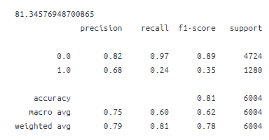

변수 선택해서 모델링한 것은 다음과 같습니다.
dummy_x = pd.get_dummies(out_X)
dummy_test_x = pd.get_dummies(test_X)

def roc_curve_plot(model, x , y ) :
    preds = model.predict_proba(x)[:,1]
    fpr, tpr, threshold = roc_curve(y, preds)
    roc_auc = auc(fpr, tpr)
    plt.figure(figsize=(10,8))
    plt.title('Receiver Operator Characteristic')
    plt.plot(fpr, tpr, 'b', label = 'AUC = {}'.format(round(roc_auc, 2)))
    plt.legend(loc = 'lower right')
    plt.plot([0,1], [0,1], 'r--')
    plt.xlim([0,1])
    plt.ylim([0,1])
    plt.ylabel('True Positive Rate')
    plt.xlabel('False Positive Rate')
    plt.show()

from sklearn.ensemble import RandomForestClassifier
from sklearn.metrics import classification_report, confusion_matrix, roc_curve,auc, accuracy_score
rf_model = RandomForestClassifier(max_depth=6, n_jobs=10,n_estimators=100)
rf_model.fit(dummy_x[significant_chi], y)
#Metrics check
predictions = rf_model.predict(dummy_test_x[significant_chi])
print(accuracy_score(testy, predictions)*100)
print(classification_report(testy,predictions))

roc_curve_plot(rf_model , dummy_test_x[significant_chi], testy)

!!!!!!!!!!!!!!!!!!!!!!!
차이가 거의 없습니다....
머 여기에는 알고리즘을 적절하지 못한 걸 사용한 것도 있을 수 있고, 연속형으로 있는 것을 괜히 binning을 해서 정보 손실이 왔을 수도 있습니다.
일단은 그래도 배울 점이나 신기한 점은 다음과 같습니다.
- 보통 one-hot을 하고 나서, 모든 데이터를 사용하는데, 차원의 저주를 해결하기 위해 그중에서도 선별했다는 것이 신기합니다. 이렇게 하는 것은 사실 처음 봤고, 보통 테스트 데이터를 안 보고 모델링하는 것이니 괜찮아 보이기도 하고, 괜히 가짓수를 줄이는 것 같기도 합니다.
https://towardsdatascience.com/categorical-feature-selection-via-chi-square-fc558b09de43
Categorical Feature Selection via Chi-Square
Analyze and selecting your categorical features for creating a prediction model
towardsdatascience.com
'분석 Python > Data Preprocessing' 카테고리의 다른 글
| Data Preprocessing 잡생각 (0) | 2020.04.19 |
|---|---|
| 텐서플로우에서 범주형 데이터 다루기 (0) | 2020.04.05 |
| [변수 선택] Python에서 변수 전처리 및 변형 해주는 Xverse 패키지 소개 (1) | 2020.03.22 |
| [실험] 정형데이터에서 연속형 변수 전처리에 따른 Network 성능 차이는 얼마나 날까? (0) | 2020.03.21 |
| [변수 선택] sklearn에 있는 mutual_info_classif , mutual_info_regression를 활용하여 변수 선택하기 (feature selection) (0) | 2020.03.09 |