
요즘은 예전만큼 모델 개발을 할 일이 없다보니, 크게 업데이트 된 것을 확인하고 싶었는데, 많은 기능이 추가되고, 이것보다 transformers 라이브러리 연습을 하는 게 더 좋을 것 같아 간단히 작성해봅니다.
버전 히스토리 (oo.ai) - 250426 기준
다음은 PyTorch 2.x 버전대 (2.0 ~ 2.7) 주요 업데이트 내용을 테이블 형태로 정리한 것입니다.
| 버전 | 주요 특징 | 세부 내용 |
| 2.0 | TorchDynamo, AOT Autograd, Distributed Tensor Parallelism (Beta) |
|
| 2.1 | torch.compile 안정화, torch.export (Prototype), Distributed Checkpointing (Prototype) |
|
| 2.2 | torch.compile 개선, FSDP (Fully Sharded Data Parallel) 성능 향상, 새로운 Python Custom Operator API |
|
| 2.3 | torch.compile 사용자 정의 Triton 커널 지원, Tensor Parallelism 기능 강화 |
|
| 2.4 | Python 3.12 지원, AOTInductor freezing, TCPStore 백엔드 전환 |
|
| 2.5 | SDPA CuDNN 백엔드, torch.compile 영역 컴파일, TorchInductor CPU 백엔드 최적화 |
|
| 2.6 | torch.compiler.set_stance, Python 3.13 지원, AOTInductor 개선, FP16 X86 CPU 지원 |
|
| 2.7 | NVIDIA Blackwell 아키텍처 지원, Torch Function Modes 지원, Mega Cache, FlexAttention |
|
설치 환경
- CUDA 12.8
- UV 사용
- 우분투
UV 설치
#!/bin/bash

# uv 설치
curl -LsSf https://astral.sh/uv/install.sh | sh

# ~/.bashrc에 ~/.local/bin을 PATH에 추가하는 라인 삽입
if ! grep -q 'export PATH="$HOME/.local/bin:$PATH"' ~/.bashrc; then
  echo 'export PATH="$HOME/.local/bin:$PATH"' >> ~/.bashrc
  echo 'PATH 설정이 ~/.bashrc에 추가되었습니다.'
else
  echo 'PATH 설정이 이미 ~/.bashrc에 존재합니다.'
fi

# 현재 세션에 PATH 변경사항 적용
export PATH="$HOME/.local/bin:$PATH"
source ~/.bashrc   # 또는 source ~/.zshrc

# uv 버전 확인
uv --version
프로젝트 설정
#!/bin/bash

uv init --python 3.10 my-pytorch-project
cd my-pytorch-project
uv venv
패키지 설치
#!/bin/bash

sudo apt update
sudo apt install build-essential

# install graphviz
sudo apt-get install graphviz
dot -V

uv add torch==2.7.0 torchvision==0.22.0 torchaudio==2.7.0
Requirements.txt
uv add -r requirements.txtipykernel
pandas
numpy
matplotlib
seaborn
scikit-learn
scipy
코드
torch.compile
torch.compile은 PyTorch 2.0에서 도입된 기능으로, 기존의 eager 모드에서 실행되는 PyTorch 코드를 TorchDynamo와 TorchInductor를 활용하여 JIT 컴파일함으로써 성능을 향상시킵니다. 이를 통해 연산 병합(fusion), 커널 최적화 등을 자동으로 수행하여 실행 속도를 높일 수 있습니다.
import torch
import torch.nn as nn

# 간단한 모델 정의
class SimpleModel(nn.Module):
    def __init__(self):
        super().__init__()
        self.linear = nn.Linear(10, 10)

    def forward(self, x):
        return torch.relu(self.linear(x))

model = SimpleModel()

# 모델 컴파일
compiled_model = torch.compile(model)

# 입력 데이터
input_data = torch.randn(1, 10)

# 컴파일된 모델 실행
output = compiled_model(input_data)
print(output)
이번에 오랜만에 보게 되니 다양하게 특정할 수 있게 하는 함수들이 많이 생긴 것 같다.
compile 전 후로 비교했을 때 성능이 개선되는 것을 확인함
start_event = torch.cuda.Event(enable_timing=True)
end_event = torch.cuda.Event(enable_timing=True)
torch.cuda.reset_peak_memory_stats()

start_event.record()
with torch.autocast(device_type='cuda', dtype=torch.float16):
    output = model(input_data)
end_event.record()


torch.cuda.synchronize()

print(f"No Compiled Elapsed time: {start_event.elapsed_time(end_event)} ms")
print(f"No Compiled Memory: {torch.cuda.max_memory_allocated() / 1024**2} MB")
torch.cuda.reset_peak_memory_stats()

start_event.record()
with torch.autocast(device_type='cuda', dtype=torch.float16):
    output = compiled_model(input_data)
end_event.record()
torch.cuda.synchronize()
print(f"Compiled Elapsed time: {start_event.elapsed_time(end_event)} ms")
print(f"Compiled Memory: {torch.cuda.max_memory_allocated() / 1024**2} MB")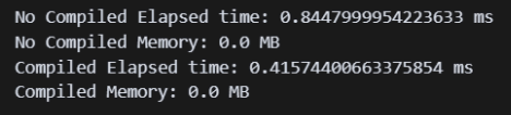
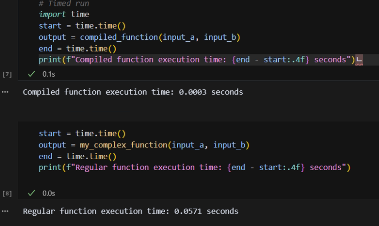
특정 함수만 최적화하는 것도 가능합니다.
import torch

# Define a regular Python function using PyTorch operations
def my_complex_function(a, b):
    x = torch.sin(a) + torch.cos(b)
    y = torch.tanh(x * a)
    return y / (torch.abs(b) + 1e-6)

# Compile the function
compiled_function = torch.compile(my_complex_function)

# Use the compiled function - first run might be slower due to compilation
input_a = torch.randn(1000, 1000).cuda() # Best results often on GPU
input_b = torch.randn(1000, 1000).cuda()

# Warm-up run (optional, but good practice for timing)
_ = compiled_function(input_a, input_b)

# Timed run
import time
start = time.time()
output = compiled_function(input_a, input_b)
end = time.time()
print(f"Compiled function execution time: {end - start:.4f} seconds")
start = time.time()
output = my_complex_function(input_a, input_b)
end = time.time()
print(f"Regular function execution time: {end - start:.4f} seconds")
컴파일 전후에 따라서 성능 차이가 나는 것을 확인하였습니다.
Utils
benchmark
새롭게 보니 벤치마크로 테스트 하는 기능이 제공되는 것을 확인하였습니다.
import torch.utils.benchmark as benchmark

t0 = benchmark.Timer(
    stmt='compiled_model(input_data)',
    globals={'compiled_model': compiled_model, 'input_data': input_data}
)

print(t0.timeit(100))
추론 방식 ( no_grad , inference_mode)
이번에 다시 보니 inference_mode라는 것이 있는 것을 보게 되었고 먼가 더 개선이 됬다고 하니 나중에 사용해봐야겠다.
- model.eval()
- 모델을 평가 모드로 전환하여 특정 레이어의 동작 변경 추론 전에 항상 호출
- torch.no_grad()
- 그래디언트 계산 비활성화 추론 시 사용 (PyTorch 1.9 미만)
- torch.inference_mode()
- 그래디언트 계산 및 내부 추적 비활성화로 성능 향상 추론 시 권장 (PyTorch 1.9 이상)
그렇다고 항상 더 빠른 것은 아닌 것 같음을 확인하였습니다.
torch.cuda.reset_peak_memory_stats()

start_event.record()
with torch.no_grad() :
    output_no_grad = compiled_model(input_data)
end_event.record()
torch.cuda.synchronize()
print(f"No Compiled Elapsed time: {start_event.elapsed_time(end_event)} ms")
print(f"No Compiled Memory: {torch.cuda.max_memory_allocated() / 1024**2} MB")
torch.cuda.reset_peak_memory_stats()

start_event.record()
with torch.inference_mode() :
    output_inference_mode = compiled_model(input_data)
end_event.record()
torch.cuda.synchronize()
print(f"Compiled Elapsed time: {start_event.elapsed_time(end_event)} ms")
print(f"Compiled Memory: {torch.cuda.max_memory_allocated() / 1024**2} MB")
Use Channels-Last Memory Format for CNNs
channels_last는 텐서의 메모리 저장 방식을 변경하여 채널 차원이 가장 안쪽에 오도록 합니다.
이는 연산 시 채널 데이터를 연속적으로 접근할 수 있게 하여 캐시 효율성과 병렬 처리 성능을 높입니다.
import torch
import torch.nn as nn

N, C, H, W = 32, 3, 224, 224 # Example dimensions
model = nn.Conv2d(C, 64, kernel_size=3, stride=1, padding=1).cuda()
input_tensor = torch.randn(N, C, H, W).cuda()

# Convert model and input to channels-last
model = model.to(memory_format=torch.channels_last)
input_tensor = input_tensor.to(memory_format=torch.channels_last)

print(f"Model parameter memory format: {model.weight.stride()}") # Stride indicates memory layout
print(f"Input tensor memory format: {input_tensor.stride()}")

# Perform operations - PyTorch handles the format internally
output = model(input_tensor)
print(f"Output tensor memory format: {output.stride()}")
Model parameter memory format: (27, 1, 9, 3)
Input tensor memory format: (150528, 1, 672, 3)
Output tensor memory format: (3211264, 1, 14336, 64)
시간을 측정해봤을 때 변환을 해서 계산하는 방식이 메모리는 더 들지만, 속도는 더 빨라지는 것을 확인하였습니다.
import torch
import torch.nn as nn
import time

# 입력 데이터 생성
N, C, H, W = 32, 3, 224, 224
input_tensor = torch.randn(N, C, H, W).cuda()
input_cl = input_tensor.to(memory_format=torch.channels_last)

# 모델 정의
model = nn.Conv2d(C, 64, kernel_size=3, stride=1, padding=1).cuda()
model_cl = nn.Conv2d(C, 64, kernel_size=3, stride=1, padding=1).cuda()
model_cl = model_cl.to(memory_format=torch.channels_last)
# 성능 측정 함수
def measure_time(model, input_tensor):
    torch.cuda.reset_peak_memory_stats()
    torch.cuda.synchronize()
    start_event.record()
    with torch.inference_mode():
        for _ in range(100):
            _ = model(input_tensor)
    end_event.record()
    torch.cuda.synchronize()
    peak_memory = torch.cuda.max_memory_allocated() / (1024 ** 2)  # MB 단위
    print(f"Peak Memory: {peak_memory:.4f} MB")
    print(f"Elapsed time: {start_event.elapsed_time(end_event)} ms")


# 성능 측정
measure_time(model, input_tensor)
measure_time(model_cl, input_cl)
Perform Graph Surgery where Required
torch.fx는 PyTorch 모델을 그래프 형태로 변환하여 분석하고 최적화할 수 있는 도구입니다. 이를 통해 모델의 구조를 시각화하거나, 특정 연산을 다른 연산으로 대체하는 등의 변형이 가능합니다.
torch.fx.symbolic_trace와 fx.GraphModule의 차이점
torch.fx.symbolic_trace: 주어진 nn.Module을 추적하여 연산 그래프를 생성하고, 이를 기반으로 새로운 GraphModule을 반환합니다. 이 과정에서 모델의 연산 흐름을 캡처하여 그래프 형태로 표현합니다.
fx.GraphModule: symbolic_trace의 결과로 생성되는 객체로, 추적된 그래프와 원래의 모듈 속성(파라미터 등)을 포함합니다. 일반적인 nn.Module처럼 사용할 수 있으며, 추적된 그래프를 기반으로 동작합니다.
즉, symbolic_trace는 모델을 추적하여 GraphModule을 생성하는 함수이며, GraphModule은 추적된 그래프와 원래 모듈의 속성을 포함하는 새로운 모듈입니다.
import torch
import torch.fx as fx

class SimpleNet(torch.nn.Module):
    def __init__(self):
        super().__init__()
        self.linear = torch.nn.Linear(5, 5)

    def forward(self, x):
        x = self.linear(x)
        x = torch.relu(x)
        return x

module = SimpleNet()
symbolic_traced : fx.GraphModule = fx.symbolic_trace(module)

# Print the traced graph representation
print("--- FX Graph ---")
print(symbolic_traced.graph)

# Print the generated Python code from the graph
print("\n--- FX Code ---")
print(symbolic_traced.code)
--- FX Graph ---
graph():
%x : [num_users=1] = placeholder[target=x]
%linear : [num_users=1] = call_module[target=linear](args = (%x,), kwargs = {})
%relu : [num_users=1] = call_function[target=torch.relu](args = (%linear,), kwargs = {})
return relu
--- FX Code ---
def forward(self, x):
linear = self.linear(x); x = None
relu = torch.relu(linear); linear = None
return relu
간단한 모델에 대한 그래프
import torch
import torch.nn as nn
from torch.fx import symbolic_trace
from torch.fx.passes.graph_drawer import FxGraphDrawer

# 간단한 모델 정의
class SimpleNet(nn.Module):
    def __init__(self):
        super().__init__()
        self.linear = nn.Linear(5, 5)

    def forward(self, x):
        x = self.linear(x)
        x = torch.relu(x)
        return x

# 모델 인스턴스 생성 및 그래프 추출
model = SimpleNet()
traced = symbolic_trace(model)

# 그래프 시각화
drawer = FxGraphDrawer(traced, 'SimpleNet')
dot_graph = drawer.get_dot_graph()
dot_graph.write_svg('simple_net_graph.svg')  # SVG 파일로 저장
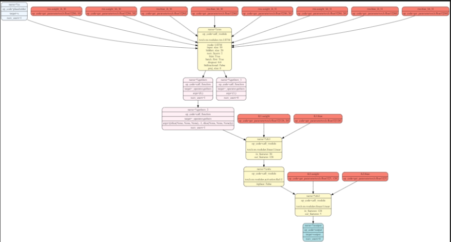
복잡한 모델에 대한 그래프
좀 더 복잡한 구조를 만들어서 해봤을 때도 그래프로 잘 표현됨을 확인하였습니다.
import torch
import torch.nn as nn

class RNN_DNN_Model(nn.Module):
    def __init__(self, input_size, hidden_size, num_layers, output_size):
        super(RNN_DNN_Model, self).__init__()
        self.rnn = nn.LSTM(input_size, hidden_size, num_layers, batch_first=True)
        self.fc1 = nn.Linear(hidden_size, 128)
        self.relu = nn.ReLU()
        self.fc2 = nn.Linear(128, output_size)

    def forward(self, x):
        out, _ = self.rnn(x)
        out = out[:, -1, :]  # 마지막 타임스텝의 출력
        out = self.fc1(out)
        out = self.relu(out)
        out = self.fc2(out)
        return out

from torch.fx import symbolic_trace
from torch.fx.passes.graph_drawer import FxGraphDrawer

# 모델 인스턴스 생성
model = RNN_DNN_Model(input_size=10, hidden_size=20, num_layers=2, output_size=5)

# 모델 추적
traced = symbolic_trace(model)

# 그래프 시각화
drawer = FxGraphDrawer(traced, 'RNN_DNN_Model')
dot_graph = drawer.get_dot_graph()
dot_graph.write_svg('rnn_dnn_model_graph.svg')  # SVG 파일로 저장
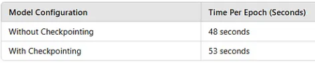
Activation Checkpointing의 작동 방식

기본 동작: 일반적으로는 순전파 시 모든 중간 활성화 값을 저장하여 역전파 시 사용합니다.
Checkpointing 적용 시: 특정 부분의 순전파에서 중간 활성화 값을 저장하지 않고, 역전파 시 해당 부분을 다시 계산하여 필요한 값을 얻습니다.
이러한 방식으로 메모리 사용량을 줄일 수 있으며, 특히 GPU 메모리가 제한된 환경에서 큰 모델을 학습할 때 유리합니다.
import torch
import torch.nn as nn
from torch.utils.checkpoint import checkpoint

# 예시 모듈 정의
class MyModule(nn.Module):
    def __init__(self):
        super().__init__()
        self.linear = nn.Linear(1000, 1000)
        self.relu = nn.ReLU()

    def forward(self, x):
        return self.relu(self.linear(x))

# 모델 인스턴스 생성
model = MyModule()

# 입력 데이터 생성
input_tensor = torch.randn(64, 1000, requires_grad=True)

# 체크포인트 적용
output = checkpoint(model, input_tensor)

# 손실 계산 및 역전파
loss = output.sum()
loss.backward()
import torch
from torch import nn
from torch.utils.checkpoint import checkpoint

class TransformerBlock(nn.Module):
    def __init__(self, embed_size):
        super().__init__()
        self.attention = nn.MultiheadAttention(embed_size, num_heads=8)
        self.feed_forward = nn.Sequential(
            nn.Linear(embed_size, embed_size * 4),
            nn.ReLU(),
            nn.Linear(embed_size * 4, embed_size)
        )

    def forward(self, x):
        # Self-attention block
        attn_output, _ = self.attention(x, x, x)
        # Adding checkpointing to the feed-forward block
        x = x + checkpoint(self.feed_forward, attn_output)
        return x

# Example usage
embed_size = 512
seq_length = 64
batch_size = 8

transformer_block = TransformerBlock(embed_size).cuda()
x = torch.randn(seq_length, batch_size, embed_size).cuda()
output = transformer_block(x)

print(f"Output Shape: {output.shape}")

import torch
from torch.cuda.amp import GradScaler, autocast
from torch.utils.checkpoint import checkpoint

class SimpleModel(nn.Module):
    def __init__(self):
        super().__init__()
        self.layer1 = nn.Linear(1024, 1024)
        self.layer2 = nn.Linear(1024, 1024)

    def forward(self, x):
        x = checkpoint(self.layer1, x)
        x = self.layer2(x)
        return x

# Instantiate model
model = SimpleModel().cuda()
optimizer = torch.optim.Adam(model.parameters())
scaler = GradScaler()

# Training loop
for epoch in range(5):
    x = torch.randn(16, 1024).cuda()

    with autocast():
        output = model(x)
        loss = output.sum()

    optimizer.zero_grad()
    scaler.scale(loss).backward()
    scaler.step(optimizer)
    scaler.update()
AMP 여부에 따른 학습 성능 및 메모리

import torch
import torch.nn as nn
import torch.optim as optim
from torchvision import datasets, transforms, models
from torch.cuda.amp import autocast, GradScaler
import time

def train_model(use_amp):
    # 데이터 전처리 및 로더 설정
    transform = transforms.Compose([
        transforms.Resize(224),
        transforms.ToTensor(),
    ])

    train_dataset = datasets.CIFAR10(root='./data', train=True,
                                     download=True, transform=transform)
    train_loader = torch.utils.data.DataLoader(train_dataset, batch_size=64,
                                               shuffle=True, num_workers=2)

    # 디바이스 설정
    device = torch.device("cuda" if torch.cuda.is_available() else "cpu")

    # 모델, 손실 함수, 옵티마이저 정의
    model = models.resnet18(pretrained=False, num_classes=10).to(device)
    criterion = nn.CrossEntropyLoss()
    optimizer = optim.SGD(model.parameters(), lr=0.01)

    # AMP 및 GradScaler 설정
    scaler = GradScaler(enabled=use_amp)

    # 학습 루프
    monitor_list = []
    start_time = time.time()
    for epoch in range(5):
        model.train()
        epoch_loss = 0
        epoch_n = 0
        torch.cuda.reset_peak_memory_stats()
        for inputs, labels in train_loader:
            inputs, labels = inputs.to(device), labels.to(device)

            optimizer.zero_grad()
            if use_amp:
                with autocast():
                    outputs = model(inputs)
                    loss = criterion(outputs, labels)
                scaler.scale(loss).backward()
                scaler.step(optimizer)
                scaler.update()
            else:
                outputs = model(inputs)
                loss = criterion(outputs, labels)
                loss.backward()
                optimizer.step()

            epoch_loss += loss.item()
            epoch_n += 1
        monitor_list.append(epoch_loss / epoch_n)
        print(f"Epoch {epoch+1} 완료")
    end_time = time.time()

    # 메모리 사용량 측정
    max_memory = torch.cuda.max_memory_allocated() / (1024 ** 2)  # MB 단위

    # 결과 출력
    print(f"총 학습 시간: {end_time - start_time:.2f}초")
    print(f"최대 GPU 메모리 사용량: {max_memory:.2f} MB")
    print("에폭별 평균 손실:", monitor_list)

# AMP 및 GradScaler 사용
print("AMP 및 GradScaler 사용:")
train_model(use_amp=True)

# AMP 및 GradScaler 미사용
print("\nAMP 및 GradScaler 미사용:")
train_model(use_amp=False)
학습 성능은 거의 비슷하게 유지하지만, 속도나 메모리 사용량에 있어서 절약해서 학습할 수 있음을 확인하였습니다.

결론
오랜만에 torch 업데이트 된 내용을 보고 정리하게 되었는데 이것 이외에도 굉장히 많은 업데이트가 된 것 같습니다.
이렇게 새로 나온 내용들은 아무래도 RAG없이는 기존 모델에게 기대할 수 없기 때문에 항상 관심있게 봐야할 것 같고, 요즘 너무 빨리 변하기 때문에 실무자 입장에서 이런 관련 문서들을 RAG 데이터로 어떻게 쉽게 만들어서 사용하게 할 수 있을 지가 중요할 것 같습니다.
참고 자료
| 제목 | 링크 |
| PyTorch Activation Checkpointing: Complete Guide | https://medium.com/@heyamit10/pytorch-activation-checkpointing-complete-guide-58d4f3b15a3d |
| Train Large ML Models With Activation Checkpointing | https://blog.dailydoseofds.com/p/train-large-ml-models-with-activation |
| PyTorch — A Comprehensive Performance Tuning Guide | https://medium.com/gitconnected/pytorch-a-comprehensive-performance-tuning-guide-a917d18bc6c2 |
| How To Train Your PyTorch Models (Much) Faster | https://levelup.gitconnected.com/how-to-train-your-pytorch-models-much-faster-14737c8c9770 |
| 2.x overview | https://pytorch.org/get-started/pytorch-2.0/ |
'분석 Python > Pytorch' 카테고리의 다른 글
| TimeSeries) [MultiHead Self Attention] multi target 예측 (0) | 2023.09.23 |
|---|---|
| Pytorch) 모델 가중치 로드 시 테스트 (전체 모델에서 서브 모델 가중치만 가져오기) (0) | 2023.09.15 |
| Pytorch) multioutput Regression 구현해보기 (4) | 2022.03.26 |
| torchfunc) titanic data에 model parallel training 해보기 (0) | 2022.03.26 |
| Pytorch 1.11 이후) functorch 알아보기 (0) | 2022.03.14 |